Branch Predictors

I have been learning about branch predictors as part of UIUC's Computer System Organization course and I thought it would be an interesting and useful exercise to build an interactive branch-prediction simulator. In particular, I wanted to simulate global history correlating branch predictors, which I will attempt to explain in this post.

I won't cover the simulator itself (IBP) in much depth here; that project has its own documentation and homepage. This post will explain the behavior of a few different branch predictors and motivate some of the features and design choices of IBP.

I will assume that readers (you) are familiar with C and understand how C programs map (roughly) to machine instructions. If not, try messing around in the Compiler Explorer and write a few assembly programs to get a feel for what's happening under the hood.

If you already know what global history correlating branch predictors are and just want to read about IBP, skip to the IBP section.

Before examining branch predictors, it's important to understand why branch prediction is useful.

A Bird's Eye View of Pipelining and ILP

The typical "Programming 101" model of computing assumes that CPUs are fed instructions one at a time and execute them in the order they appear in the program. This is usually incorrect in two important ways:

1. CPUs are pipelined: they read and execute instructions in multiple stages, which allows them to read new instructions while executing older ones.
2. CPUs execute multiple instructions in parallel and can complete them out-of-order, which means newer instructions can finish executing before older ones. (Instruction Level Parallelism a.k.a ILP)

Different CPUs have different degrees of parallelism and different pipeline architectures. What this boils down to is that CPU designers try to leverage the inherent parallelism of hardware to speed up the execution of sequential programs as much as possible.

Branch instructions (among other things -- data hazards, structural hazards, memory operations, etc.) often throw a wrench into this pursuit of speed through parallelism. Consider the following branch-less program:

main:
  add r1, r2, r6   // r1 = r2 + r6
  mul r3, r2, r3   // r3 = r2 * r3
  sub r4, r4, r2   // r4 = r4 - r2
  add r5, r5, r6   // r5 = r5 + r6

We can execute these four instructions in any order without changing their behavior. This means that CPUs can execute them in parallel or out-of-order to speed up the whole program.

What if we replaced the sub instruction with a conditional branch?

main:
  add r1, r2, r6              // r1 = r2 + r6
  mul r3, r2, r3              // r3 = r2 * r3
  beq r6, r7, somewhere_else  // if (r6 == r7) goto somewhere_else
  add r5, r5, r6              // r5 = r5 + r6

somewhere_else:
  // some code here

This creates two complications:

1. We can't reorder instructions "across" the branch: everything that's above the branch stays above it, and everything that's below the branch stays below it.
2. We don't know what to execute after the branch until we've executed the branch.

This severely limits the CPU's ability to speed up the program through dynamic scheduling and ILP unless we can predict sufficiently in advance whether the branch is taken or not.

This is the basic problem that branch predictors aim to solve. An ideal branch predictor which achieves 100% prediction accuracy would allow us to parallelize execution around branch instructions like any other instruction.

Of course, no predictor is 100% accurate so we need to be able to deal with mispredictions. This is typically done by "flushing" instructions on the wrong branch path, i.e aborting execution before they can write to registers or cause other side effects. How this is implemented depends on the structure of the CPU pipeline and other elements of the microarchitecture, so I will not cover it here. Mispredicting and flushing instructions is generally no more expensive than not predicting at all, so branch prediction is strictly beneficial to runtime and CPU resource utilization.

Example

To get a better sense of the impact of branch prediction, let's look at two variants of a simple program.

First, the "random" branching variant:

#include <stdio.h>
#include <stdlib.h>
#include <time.h>

int main()
{
  srand(time(NULL));
  int count = 0;
  for (int i = 0; i < 10000000; ++i)
  {
    int n = rand();
    if (n % 2 == 0) ++count; // <-- this branch is "random"
  }
  printf("%d\n", count);
  return 0;
}

Second, the predictable variant:

#include <stdio.h>
#include <stdlib.h>
#include <time.h>

int main()
{
  srand(time(NULL));
  int count = 0;
  for (int i = 0; i < 10000000; ++i)
  {
    int n = rand();
    if (i % 2 == 0) ++count; // <-- this branch behaves predictably
  }
  printf("%d\n", count);
  return 0;
}

Compiling these programs with -O0 (one and two) we see two conditional branch instructions: one corresponding with the loop and another corresponding with the if statement. Since the loop branch is almost always not taken (i.e execution continues in the loop body) we will assume that the branch predictor is able to achieve near-perfect accuracy on this branch.

The if-statement branch is more interesting. In the random variant, no predictor will be more or less accurate than 50%. In the predictable variant, a smart enough predictor should achieve nearly 100% accuracy. Running an unscientific test on my 1.6GHz Intel i5 MacBook Air, I observed the random branching program take ~2x as long as the predictable one.

testing consistent branches
5000000

real 0m0.081s user 0m0.077s sys 0m0.002s
5000000
real 0m0.075s user 0m0.071s sys 0m0.002s
5000000
real 0m0.075s user 0m0.072s sys 0m0.002s
5000000
real 0m0.075s user 0m0.072s sys 0m0.002s
5000000
real 0m0.075s user 0m0.071s sys 0m0.002s
5000000
real 0m0.076s user 0m0.073s sys 0m0.002s
5000000
real 0m0.079s user 0m0.074s sys 0m0.002s
5000000
real 0m0.078s user 0m0.073s sys 0m0.002s
5000000
real 0m0.083s user 0m0.078s sys 0m0.002s
5000000
real 0m0.075s user 0m0.072s sys 0m0.002s
5000000
real 0m0.076s user 0m0.073s sys 0m0.002s
testing random branches 5001674
real 0m0.164s user 0m0.158s sys 0m0.003s
5001674
real 0m0.160s user 0m0.156s sys 0m0.002s
5001674
real 0m0.159s user 0m0.156s sys 0m0.002s
5001674
real 0m0.163s user 0m0.159s sys 0m0.002s
5001674
real 0m0.160s user 0m0.155s sys 0m0.002s
5001674
real 0m0.160s user 0m0.156s sys 0m0.002s
5001674
real 0m0.161s user 0m0.157s sys 0m0.002s
4999206
real 0m0.161s user 0m0.157s sys 0m0.002s
4999206
real 0m0.160s user 0m0.156s sys 0m0.002s
4999206
real 0m0.160s user 0m0.156s sys 0m0.002s
4999206
real 0m0.162s user 0m0.158s sys 0m0.002s 

Static Predictors

These are the simplest branch predictors; they always make the same prediction for each branch instruction and do not account for the behavior of the program at runtime (hence "static"). Early MIPS processors implemented single-direction static prediction by always predicting that conditional branches are not taken. A more advanced form of static prediction would be to predict that forward branches are not taken and backwards branches are or vice-versa. Regardless of the type of static predictor, all static predictions are known at compile time.

Static predictors generally perform worse than dynamic predictors, which use the runtime history of each branch to make predictions.

1-bit Predictor

This is the simplest form of dynamic branch prediction. This predictor makes a prediction for each branch instruction based on the previous execution of that branch instruction.

In the most common implementation: if a particular branch instruction is taken then it will be predicted taken the next time it is executed; if it is not taken then it will be predicted not taken the next time it is executed.

This predictor is usually implemented as a hash table whose keys are the program counter (a.k.a instruction pointer) values at each branch instruction and whose values are a single bit representing the last direction (taken or not taken) for that branch. The "hash function" is typically just truncating the PC to its lowest 2 / 4 / 8 / etc. bits depending on the size of the table.

For example,

loop:
  // ...
  beq r1, r2, label   // Branch 1: PC = 0b00001101, NOT TAKEN this iteration
  // ...
  bne r4, r5, label2  // Branch 2: PC = 0b00010111, NOT TAKEN this iteration
  // ...
  beq r3, r4, label3  // Branch 3: PC = 0b00101100, TAKEN this iteration
  // ...
  bgt r5, r6, label4  // Branch 4: PC = 0b00111110, TAKEN this iteration
  // ...
  jmp loop            // Loop

The predictor table looks like this after the first iteration of the loop:

In the second iteration, branches 3 and 4 would be predicted taken and branches 1 and 2 would be predicted not taken. Every time a branch instruction is executed, the corresponding table entry is updated with the direction of the branch.

Of course, one of the problems with this predictor is aliasing: different PCs can map to the same table entries if they have the same least significant bits. This is unavoidable since the predictor table is a fixed-size piece of hardware so I won't focus too much on mitigating it. What is more interesting is the behavior of the predictor on common program patterns and on some "pathological" programs.

Unsurprisingly, this predictor performs very well with branches that don't "flip" frequently, such as loops. One pathological program that stumps it is the "predictable" test program I used earlier:

// ...
  for (int i = 0; i < 10000000; ++i)
  {
    // ...
    if (i % 2 == 0) ++count; // <-- this branch behaves predictably
  }
// ...

Assuming no aliasing, this predictor would achieve 0% accuracy on the if-statement branch! That's even worse than a static predictor. Surely we can do better!

2-bit Predictors and Saturating Counters

The 2-bit predictor is a simple upgrade from the 1-bit predictor. Instead of using a table with 1-bit values, we use two bits to make predictions and update the table according to the following state machine:

The "T" and "N" edges are traversed when a branch is taken and not taken respectively. When the value in the table is 10 or 11, the branch is predicted taken; otherwise, it is predicted not taken. The example 1-bit predictor table from above would look like this with 2-bit values:

The important distinction is that all four branches would be predicted not taken in the next iteration. In effect, this predictor has a higher tolerance for "flipping": in the 00 state, it requires a branch to be taken twice to change the prediction to "taken" (10), and behaves similarly (but in the opposite direction) in the 11 state.

This predictor performs much better on the pathological if-branch that stumped the 1-bit predictor: it achieves 50% accuracy, which is at least on par with a static predictor. It should be fairly simple to come up with a similar pathological branch that defeats this predictor; I leave it as an exercise for the reader.

Saturating counters are another upgrade from the 1-bit predictor that take a different approach:

1. Maintain an n-bit counter for each branch instruction (each value in the table is n bits).
2. Increment the counter when the branch is taken and decrement when it is not taken (the value is capped on both sides to prevent overflow).
3. Predict taken if and only if the value is at least 2^n-1.

An n-bit saturating counter will predict taken (or not taken) if a branch was mostly taken (or not taken) in the past 2ⁿ executions. In practice, saturating counters perform similarly to the 2-bit FSM.

Global History Correlating Predictors

We are finally ready to tackle the subject of this post. The goal of global history predictors is to use the history of other branches to predict the next branch; global refers to all branches in the program.

This is accomplished by means of a SIPO shift register that tracks global branch history. A shift register is best described as a fixed-size queue of bits: bits are pushed one at a time into one side of the register, and the "oldest" bit is removed from the other side of the register every time a bit is pushed. SIPO shift registers can be read in parallel, which means we can read all the bits in the shift register at once (like a normal register) instead of de-queueing and reading them one at a time.

This is best explained with an example. Here is some pseudocode that lists a sequence of branch instructions and the state of the shift register after each branch:

program start
// Shift Register = 0000

taken branch
// Shift Register = 0001

not taken branch
// Shift Register = 0010

taken branch
// Shift Register = 0101

taken branch
// Shift Register = 1011

not taken branch
// Shift Register = 0110

// ...

We are assuming a 4-bit shift register, and that bits are pushed into the shift register from the "right". An n-bit shift register records the direction of the past n branches.

This predictor correlates predictions with the global branch history by using the shift register to choose one of many predictor tables. For example, with the same 4-bit shift register and program as above:

1. The predictor would have 2⁴ = 16 predictor tables, each of which has some number of 1/2/n-bit prediction entries.
2. Before the first branch instruction is executed, the value in the shift register is 0 so predictions are made with the first (i.e index 0) table. The predictor accesses an entry in this table with the lower bits of the PC of the branch instruction as in the 1 and 2-bit predictors described earlier.
3. Before the second branch instruction is executed, the value in the shift register is 2 so predictions are made with the third table.
4. The same process happens for the subsequent branch instructions and the rest of the program -- the shift register indexes a set of 16 predictor tables that are each indexed by PC.

Equivalently, the predictor could be modeled as a single large table that is indexed by the shift register concatenated with the lower bits of the PC. In both models, if the shift register is P bits long and the lowest S bits of the PC are used to index prediction tables, the predictor has a total of 2^S * 2^P = 2^{S + P} prediction entries. If each prediction entry is N bits, the total number of bits that make up the table(s) is 2^{S + P + N}. Including the size of the shift register, the total size of the predictor is 2^{S + P + N} + P bits. This term is also called the area of the predictor.

Larger area requires more hardware and is more expensive, so branch predictors are optimized for low area in addition to high accuracy.

Global history predictors that concatenate the shift register with the branch PC are called gselect predictors, and this is the type of predictor that IBP simulates. gselect predictors tend to perform better with more history bits (P) and more PC bits (S), but increasing S and P increases the number of predictor entries exponentially. Fortunately, this is not a problem for a software branch prediction simulator :)

gselect predictors are usually >90% accurate (see Table 6 here). On our "predictable" test program, a gselect predictor with 1-bit prediction entries and a 2-bit shift register would achieve 100% accuracy!

This is because the direction of the if-statement branch can be predicted from its direction in the last iteration. After a few iterations, a not-taken if-statement leads to a table where the if-statement branch entry is 1, and a taken if-statement leads to a table where the if-statement branch entry is 0.

This section is already very long so I will stop here and continue later. It is finally time to introduce IBP.

IBP: Interactive Branch Predictor

Let's examine this from left to right.

Throughout this post, I have been using the following small loop from the example program to compare predictors:

// ...
  for (int i = 0; i < 10000000; ++i)
  {
    // ...
    if (i % 2 == 0) ++count; // <-- this branch behaves predictably
  }
// ...

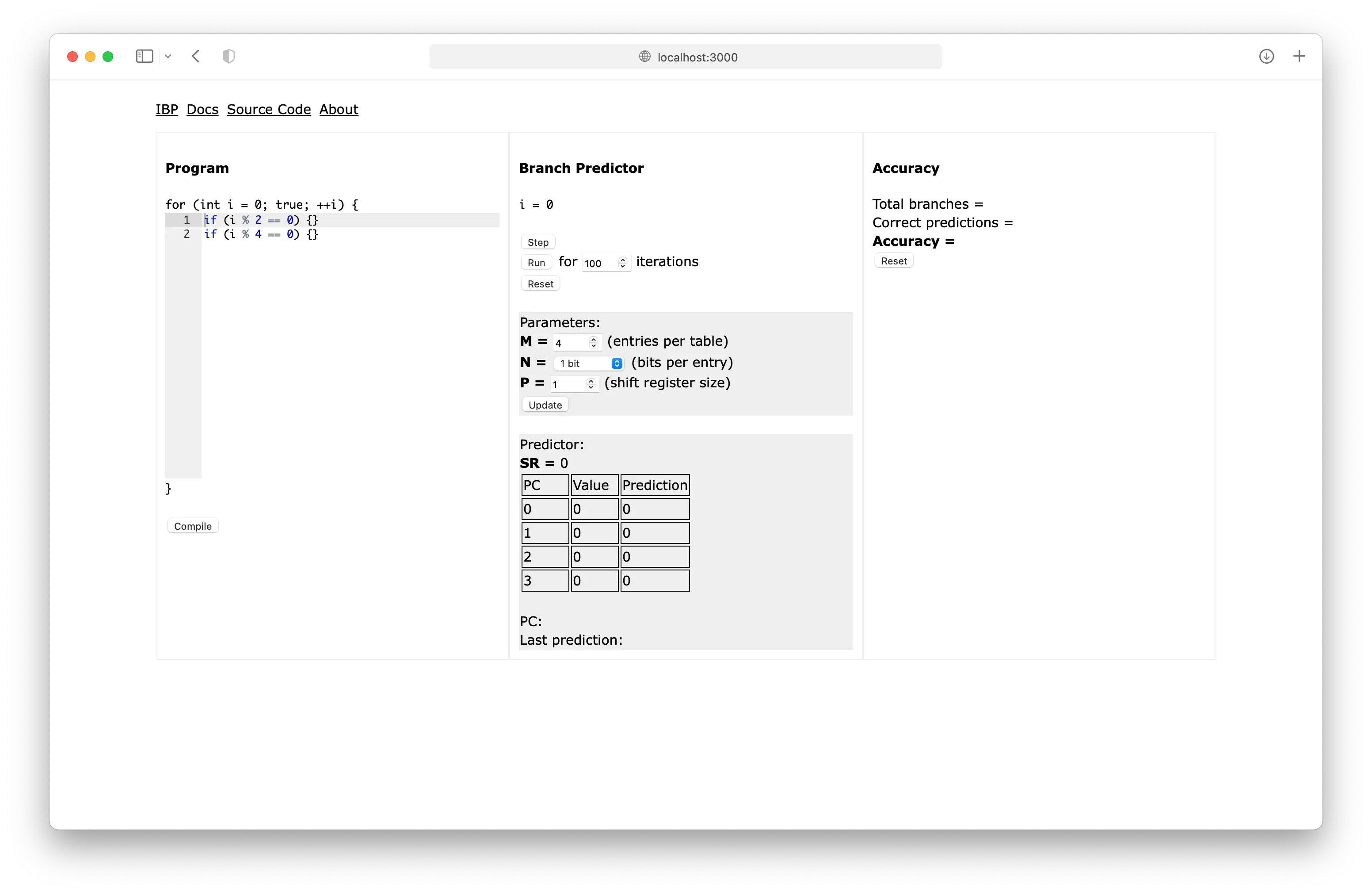
This structure -- an (effectively) infinite loop that executes the same branches repeatedly -- happens to be a great way to test branch predictors. The "Program" area of IBP represents the same kind of loop and uses a simple C-like language to describe variables and branches. IBP can perform common mathematical, logical and bitwise operations and generate pseudo-random numbers to use in if-statements, which are the branches of the program. The loop branch is omitted from the simulator since its behavior is not especially interesting.

The "Branch Predictor" area in the middle displays the state of the predictor and drives the simulation. The table displayed in the "Predictor" box is the M-entry predictor table selected by the shift register.

(Earlier I used "S" to describe the number of bits of the PC used to index the predictor table; "M" represents the same parameter of the predictor, except that M = 2^S.)

The PC of each branch instruction (i.e. if statement) is its line number as displayed in the editor. The corresponding predictor table entry of every branch instruction is at index PC % M.

Currently IBP only simulates 1-bit and 2-bit (FSM) predictor entries.

The "Accuracy" area displays the overall and per-PC accuracy of the predictor.

IBP is great for examining the behavior of branch predictors on various programs and investigating "pathological" programs that stump branch predictors. It also happens to be a useful tool for Computer Architecture coursework :)

The IBP documentation describes the interface and program language in more detail.

More About Correlating Predictors

This section is a collection of unrelated observations and facts about correlating predictors that I couldn't write too much about in the interest of concision and time.

Local predictors take a different approach to history correlation than global predictors: they have a separate history buffer for each branch, which means the prediction for each branch does not depend on the history of other branches. Local predictors generally have the same area footprint as global predictors and also perform very well.

gselect predictors concatenate history bits with the branch PC to select a predictor entry, but gshare predictors XOR the two instead; this leads to less aliasing and better performance (look at the tables here) at smaller area.

The following digression is not really relevant but I found it interesting:

When working on some branch prediction homework problems, I had conjectured with a fellow 1010labs member that adding global history correlation (i.e a shift register and more tables) to a simple 1 or 2-bit predictor would never worsen its accuracy on a given branch instruction (after the predictor has "warmed up" in the first few iterations of the loop).

This seemed intuitively obvious, since using more information to predict branches should lead to better prediction accuracy. However, this is actually false: it is possible (and not especially difficult) to construct pathological programs on which non-correlating predictors perform better than their correlating counterparts, as shown by a fellow researcher. Consider the following program:

for (int i = 0; true; ++i)
{
  if ((i + 1) % 4 < 2) {}
  if (i % 4 < 2) {} // <-- this branch an exception
}

Omitting the loop branch and considering the second if statement, a simple 1-bit predictor would achieve 50% accuracy. A 1-bit predictor with a 2-bit shift register achieves 0% accuracy -- it doesn't make a single correct prediction of this branch!

/digression

That's all for now!

Conclusion

I've written enough so I'll conclude with a few short points and some further reading:

• The source code of IBP is here.
• Matt Godbolt has written a series of interesting articles about his investigation of branch prediction on Intel processors: https://xania.org/201602/bpu-part-one
• Agner Fog has written extensively about Intel/AMD microarchitecture and branch prediction. His website is a gold mine of interesting information.
• Modern branch predictors are very very good -- consistently >90% accurate. Even static predictors can take advantage of loops and speed up execution by a lot. I would recommend writing some small predictable and unpredictable programs and testing them on your machine to see the impact of branch prediction.
• I was very surprised to learn that dynamic hardware-based predictors are on par with or better than compiler-aided static techniques. This seems obvious now but I was once a rather self-important compiler enthusiast; now I seek truth in the hardware.